
| 일 | 월 | 화 | 수 | 목 | 금 | 토 |
|---|---|---|---|---|---|---|
| 1 | 2 | 3 | 4 | 5 | ||
| 6 | 7 | 8 | 9 | 10 | 11 | 12 |
| 13 | 14 | 15 | 16 | 17 | 18 | 19 |
| 20 | 21 | 22 | 23 | 24 | 25 | 26 |
| 27 | 28 | 29 | 30 |
- Object Detection
- AP
- Multi-task loss
- Non maximum suppression
- Faster R-CNN
- Region proposal Network
- hard negative mining
- R-CNN
- multi task loss
- Fast R-CNN
- Map
- BiFPN
- YOLO
- mean Average Precision
- Detection Transformer
- Darknet
- RPN
- Average Precision
- IOU
- Object Detection metric
- detr
- pytorch
- fine tune AlexNet
- object queries
- Anchor box
- RoI pooling
- Linear SVM
- herbwood
- Bounding box regressor
- Hungarian algorithm
- Today
- Total
약초의 숲으로 놀러오세요
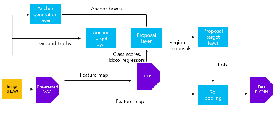
Pytorch로 구현한 Faster R-CNN 모델 본문
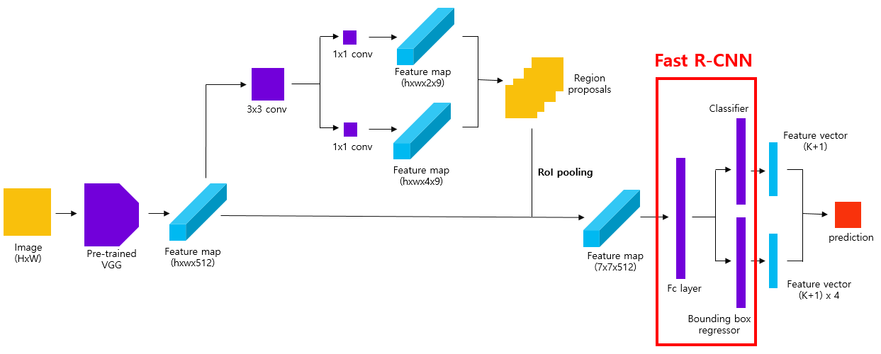
이번 포스팅에서는 How FasterRCNN works and step-by-step PyTorch implementation 영상에 올라온 pytorch로 구현한 Faster R-CNN 코드를 분석해보도록 하겠습니다. Faster R-CNN은 여러 코드 구현체가 있었지만, 살펴볼 코드가 RPN 내부에서 동작하는 여러 과정들을 직관적으로 잘 보여준 것 같아서 선정하게 되었습니다. 단일 이미지를 입력하여 Faster R-CNN 모델의 각 모듈의 입출력 데이터와 동작 과정을 쉽게 확인할 수 있습니다. 해당 모델에 대한 설명은 Faster R-CNN 논문 리뷰 포스팅을 참고하시기 바랍니다.
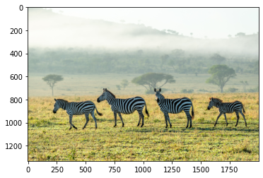
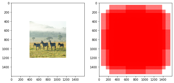
저는 입력 이미지로 위의 얼룩말 이미지를 사용했습니다. 편의를 위해 원본 이미지를 800x800 크기로 resize해주었습니다. 실제 sub-sampling ratio=1/16으로 지정하여 feature extractor를 거친 feature map의 크기는 50x50이 됩니다. 코드는 제 github repository에 정리해두었습니다.
1) Feature extraction by pre-trained VGG16
model = torchvision.models.vgg16(pretrained=True).to(DEVICE)
features = list(model.features)

# only collect layers with output feature map size (W, H) < 50
dummy_img = torch.zeros((1, 3, 800, 800)).float() # test image array

req_features = []
output = dummy_img.clone().to(DEVICE)

for feature in features:
    output = feature(output)
#     print(output.size()) => torch.Size([batch_size, channel, width, height])
    if output.size()[2] < 800//16: # 800/16=50
        break
    req_features.append(feature)
    out_channels = output.size()[1]

faster_rcnn_feature_extractor = nn.Sequential(*req_features)

output_map = faster_rcnn_feature_extractor(imgTensor)
먼저 원본 이미지에 대하여 feature extraction을 수행할 pre-trained VGG16 모델을 정의합니다. 그 다음 전체 모델에서 sub-sampling ratio에 맞게 50x50 크기가 되는 layer까지만 feature extractor로 사용합니다. 이를 위해 원본 이미지와 크기가 같은 800x800 크기의 dummy 배열을 입력하여 50x50 크기의 feature map을 출력하는 layer를 찾습니다. 이후 faster_rcnn_feature_extractor 변수에 전체 모델에서 해당 layer까지만 저장합니다. 이후 원본 이미지를 faster_rcnn_feature_extractor에 입력하여 50x50x512 크기의 feature map을 얻습니다.
2) Anchor generation layer
feature_size = 800 // 16
ctr_x = np.arange(16, (feature_size + 1) * 16, 16)
ctr_y = np.arange(16, (feature_size + 1) * 16, 16)
ratios = [0.5, 1, 2]
scales = [8, 16, 32]
sub_sample = 16
anchor_boxes = np.zeros(((feature_size * feature_size * 9), 4))
index = 0
for c in ctr: # per anchors
ctr_y, ctr_x = c
for i in range(len(ratios)): # per ratios
for j in range(len(scales)): # per scales
# anchor box height, width
h = sub_sample * scales[j] * np.sqrt(ratios[i])
w = sub_sample * scales[j] * np.sqrt(1./ ratios[i])
# anchor box [x1, y1, x2, y2]
anchor_boxes[index, 1] = ctr_y - h / 2.
anchor_boxes[index, 0] = ctr_x - w / 2.
anchor_boxes[index, 3] = ctr_y + h / 2.
anchor_boxes[index, 2] = ctr_x + w / 2.
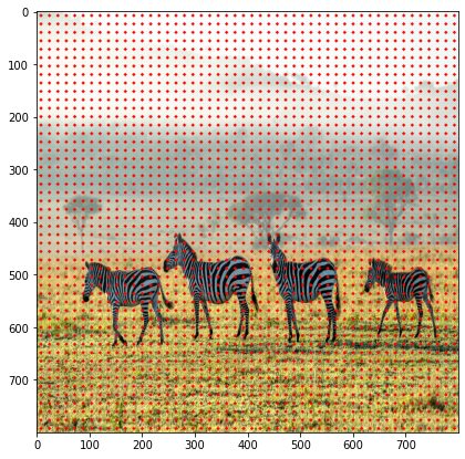
index += 1Anchor generation layer에서는 anchor box를 생성하는 역할을 합니다. 이미지의 크기가 800x800이며, sub-sampling ratio=1/16이므로, 총 22500(=50x50)개의 anchor box를 생성해야 합니다. 이를 위해 16x16 간격의 grid마다 anchor를 생성해준 후, anchor를 기준으로 서로 다른 scale과 aspect ratio를 가지는 9개의 anchor box를 생성해줍니다. anchor_boxes 변수에 전체 anchor box의 좌표(x1, y1, x2, y2)를 저장합니다(anchor_boxes 변수의 크기는 (22500, 4)입니다).
3) Anchor Target layer
index_inside = np.where(
        (anchor_boxes[:, 0] >= 0) &
        (anchor_boxes[:, 1] >= 0) &
        (anchor_boxes[:, 2] <= 800) &
        (anchor_boxes[:, 3] <= 800))[0]

valid_anchor_boxes = anchor_boxes[index_inside]
Anchor Target layer에서는 RPN을 학습시키기 위해 적절한 anchor box를 선택하는 작업을 수행합니다. 먼저 위와 같이 이미지 경계(=800x80) 내부에 있는 anchor box만을 선택합니다.
label = np.empty((len(index_inside),), dtype=np.int32)
label.fill(-1)

pos_iou_threshold = 0.7
neg_iou_threshold = 0.3

label[gt_argmax_ious] = 1
label[max_ious >= pos_iou_threshold] = 1
label[max_ious < neg_iou_threshold] = 0

n_sample = 256
pos_ratio = 0.5
n_pos = pos_ratio * n_sample

pos_index = np.where(label == 1)[0]

if len(pos_index) > n_pos:
    disable_index = np.random.choice(pos_index,
                                    size = (len(pos_index) - n_pos),
                                    replace=False)
    label[disable_index] = -1
그 다음 전체 anchor box에 대하여 ground truth box와의 IoU값을 구합니다(이 부분에 대한 설명은 생략했습니다. 원본 코드를 참고하시기 바랍니다). 그리고 각 ground truth box와 IoU가 가장 큰 anchor box와 IoU 값이 0.7 이상인 anchor box를 positive sample로, IoU 값이 0.3 미만인 anchor box는 negative sample로 저장합니다. label 변수에positive sample일 경우 1, negative sample일 경우 0으로 저장합니다.
mini-batch의 수는 256개로, positive/negative sample의 비율이 1:1이 되도록 구성합니다. 만약 positive sample의 수가 128개 이상인 경우, 남는 positive sample에 해당하는 sample은 label 변수에 -1로 지정합니다. negative sample에 대해서도 마찬가지로 수행합니다. 하지만 일반적으로 positive sample의 수가 128개 미만일 경우, 부족한만큼의 sample을 negative sample에서 추출합니다.
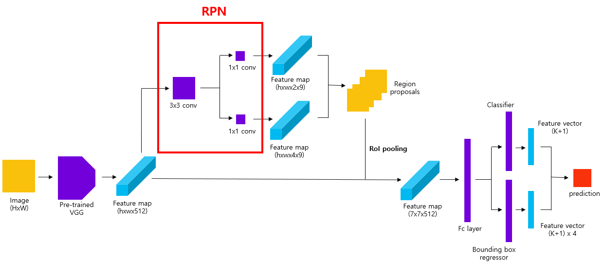
4) RPN(Region Proposal Network)
in_channels = 512
mid_channels = 512
n_anchor = 9

conv1 = nn.Conv2d(in_channels, mid_channels, 3, 1, 1).to(DEVICE)
conv1.weight.data.normal_(0, 0.01)
conv1.bias.data.zero_()

# bounding box regressor
reg_layer = nn.Conv2d(mid_channels, n_anchor * 4, 1, 1, 0).to(DEVICE)
reg_layer.weight.data.normal_(0, 0.01)
reg_layer.bias.data.zero_()

# classifier(object or not)
cls_layer = nn.Conv2d(mid_channels, n_anchor * 2, 1, 1, 0).to(DEVICE)
cls_layer.weight.data.normal_(0, 0.01)
cls_layer.bias.data.zero_()
RPN(Region Proposal Network)를 정의합니다. 1)번 과정을 통해 생성된 feature map에 3x3 conv 연산을 적용하는 layer를 정의합니다. 이후 1x1 conv 연산을 적용하여 9x4(anchor box의 수 x bounding box coordinates)개의 channel을 가지는 feature map을 반환하는 Bounding box regressor를 정의합니다. 마찬가지로 1x1 conv 연산을 적용하여 9x2(anchor box의 수 x object 여부)개의 channel을 가지는 feature map을 반환하는 Classifier를 정의합니다.
x = conv1(output_map.to(DEVICE)) # output_map = faster_rcnn_feature_extractor(imgTensor)
pred_anchor_locs = reg_layer(x) # bounding box regresor output
pred_cls_scores = cls_layer(x)  # classifier output

pred_anchor_locs = pred_anchor_locs.permute(0, 2, 3, 1).contiguous().view(1, -1, 4)
print(pred_anchor_locs.shape)

pred_cls_scores = pred_cls_scores.permute(0, 2, 3, 1).contiguous()
print(pred_cls_scores.shape)

objectness_score = pred_cls_scores.view(1, 50, 50, 9, 2)[:, :, :, :, 1].contiguous().view(1, -1)
print(objectness_score.shape)

pred_cls_scores = pred_cls_scores.view(1, -1, 2)
print(pred_cls_scores.shape)
1)번 과정에서 얻은 50x50x512 크기의 feature map을 3x3 conv layer에 입력합니다. 이를 통해 얻은 50x50x512 크기의 feature map을 Bounding box regressor, Classifier에 입력하여 각각 bounding box coefficients(=pred_anchor_locs)와 objectness score(=pred_cls_scores)를 얻습니다. 이를 target 값과 비교하기 위해 적절하게 resize해줍니다.
rpn_cls_loss = F.cross_entropy(rpn_score, gt_rpn_score.long().to(DEVICE), ignore_index = -1)

# only positive samples
pos = gt_rpn_score > 0
mask = pos.unsqueeze(1).expand_as(rpn_loc)
print(mask.shape)

# take those bounding boxes whick have positive labels
mask_loc_preds = rpn_loc[mask].view(-1, 4)
mask_loc_targets = gt_rpn_loc[mask].view(-1, 4)
print(mask_loc_preds.shape, mask_loc_targets.shape)

x = torch.abs(mask_loc_targets.cpu() - mask_loc_preds.cpu())
rpn_loc_loss = ((x < 1).float() * 0.5 * x ** 2) + ((x >= 1).float() * (x - 0.5))
print(rpn_loc_loss.sum())

rpn_lambda = 10
N_reg = (gt_rpn_score > 0).float().sum()
rpn_loc_loss = rpn_loc_loss.sum() / N_reg
rpn_loss = rpn_cls_loss + (rpn_lambda * rpn_loc_loss)
print(rpn_loss)
다음으로 RPN의 loss를 계산하는 과정을 살펴보겠습니다. Classification loss는 cross entropy loss를 활용하여 구합니다. Bounding box regression loss는 오직 positive에 해당하는 sample에 대해서만 loss를 계산하므로, positive/negative 여부를 저장하는 배열인 mask를 생성해줍니다. 이를 활용하여 Smooth L1 loss를 구해줍니다. Classification loss와 Bounding box regression loss 사이를 조정하는 balancing parameter $\lambda=10$으로 지정해주고 두 loss를 더해 multi-task loss를 구합니다.
5) Proposal layer
nms_thresh = 0.7  # non-maximum supression (NMS)
n_train_pre_nms = 12000 # no. of train pre-NMS
n_train_post_nms = 2000 # after nms, training Fast R-CNN using 2000 RPN proposals
n_test_pre_nms = 6000
n_test_post_nms = 300 # During testing we evaluate 300 proposals,
min_size = 16

order = score.ravel().argsort()[::-1]
order = order[:n_train_pre_nms]
roi = roi[order, :]

order = order.argsort()[::-1]
keep = []

while (order.size > 0):
  i = order[0] # take the 1st elt in roder and append to keep
  keep.append(i)

  xx1 = np.maximum(x1[i], x1[order[1:]])
  yy1 = np.maximum(y1[i], y1[order[1:]])
  xx2 = np.minimum(x2[i], x2[order[1:]])
  yy2 = np.minimum(y2[i], y2[order[1:]])

  w = np.maximum(0.0, xx2 - xx1 + 1)
  h = np.maximum(0.0, yy2 - yy1 + 1)

  inter = w * h
  ovr = inter / (areas[i] + areas[order[1:]] - inter)
  inds = np.where(ovr <= nms_thresh)[0]
  order = order[inds + 1]

keep = keep[:n_train_post_nms] # while training/testing, use accordingly
roi = roi[keep]
Proposal layer에서는 Anchor generation layer에서 생성된 anchor boxes와 RPN에서 반환한 class scores와 bounding box regressor를 사용하여 region proposals를 추출하는 작업을 수행합니다. 먼저 score 변수에 저장된 objectness score를 내림차순으로 정렬한 후 objectness score 상위 N(n_train_pre_nms=12000)개의 anchor box에 대하여 Non maximum suppression 알고리즘을 수행합니다. 남은 anchor box 중 상위 N(n_train_post_nms=2000)개의 region proposals를 학습에 사용합니다.
6) Proposal Target layer
n_sample = 128 # number of samples from roi
pos_ratio = 0.25 # number of positive examples out of the n_samples
# min iou of region proposal with any ground truth object
# to consider as positive sample
pos_iou_thresh = 0.5
neg_iou_thresh_hi = 0.5 # iou 0~0.5 is considered as negative (0, background)
neg_iou_thresh_lo = 0.0
(...)
gt_assignment = ious.argmax(axis=1)
max_iou = ious.max(axis=1)
print(gt_assignment)
print(max_iou)
# assign the labels to each proposal
gt_roi_label = labels[gt_assignment]
print(gt_roi_label)
pos_roi_per_image = 32
pos_index = np.where(max_iou >= pos_iou_thresh)[0]
pos_roi_per_this_image = int(min(pos_roi_per_image, pos_index.size))
if pos_index.size > 0:
pos_index = np.random.choice(
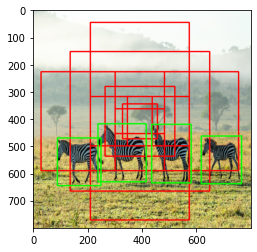
pos_index, size=pos_roi_per_this_image, replace=False)Proposal target layer의 목표는 proposal layer에서 나온 region proposals 중에서 Fast R-CNN 모델을 학습시키기 위한 유용한 sample을 선택하는 것입니다. 학습을 위해 128개의 sample을 mini-batch로 구성합니다. 이 때 Proposal layer에서 얻은 anchor box 중 ground truth box와의 IoU 값이 0.5 이상인 box를 positive sample로, 0.5 미만인 box를 negative sample로 지정합니다(IoU를 구하는 과정은 코드를 참고하시기 바랍니다). 전체 mini-batch sample 중 1/4, 즉 32개가 positive sample이 되도록 구성합니다. positive sample이 32개 미만인 경우 부족한 sample은 negative sample에서 구합니다(위의 코드에서 positive sample의 수는 21개, negative sample의 수는 107개입니다).
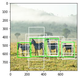
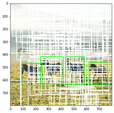
위의 그림에서 초록색 box는 ground truth box, 흰 색 box는 predicted bounding box입니다. 왼쪽 그림은 positive sample에 해당하는 box를, 오른쪽 그림은 negative sample에 해당하는 box를 시각화한 결과입니다. 왼쪽 그림에서는 얼룩말의 위치를 상대적을 잘 맞춘 반면, 오른쪽 그림에서는 다수의 box가 배경을 포함하고 있는 모습을 확인할 수 있습니다.
7) RoI pooling
rois = torch.from_numpy(sample_roi).float()
roi_indices = 0 * np.ones((len(rois),), dtype=np.int32)
roi_indices = torch.from_numpy(roi_indices).float()

indices_and_rois = torch.cat([roi_indices[:, None], rois], dim=1)
xy_indices_and_rois = indices_and_rois[:, [0, 2, 1, 4, 3]]
indices_and_rois = xy_indices_and_rois.contiguous()

size = (7, 7)
adaptive_max_pool = nn.AdaptiveMaxPool2d(size[0], size[1])

output = []
rois = indices_and_rois.data.float()
rois[:, 1:].mul_(1/16.0) # sub-sampling ratio
rois = rois.long()
num_rois = rois.size(0)

for i in range(num_rois):
  roi = rois[i]
  im_idx = roi[0]
  im = output_map.narrow(0, im_idx, 1)[..., roi[1]:(roi[3]+1), roi[2]:(roi[4]+1)]
  tmp = adaptive_max_pool(im)
  output.append(tmp[0])

output = torch.cat(output, 0)
Feature extractor를 통해 얻은 feature map과 Proposal Target layer에서 추출한 region proposals을 활용하여 RoI pooling을 수행합니다. 이 때 output feature map의 크기가 7x7이 되도록 설정합니다.
8) Fast R-CNN
roi_head_classifier = nn.Sequential(*[nn.Linear(25088, 4096), nn.Linear(4096, 4096)]).to(DEVICE)
cls_loc = nn.Linear(4096, 2 * 4).to(DEVICE) # 1 class, 1 background, 4 coordiinates
cls_loc.weight.data.normal_(0, 0.01)
cls_loc.bias.data.zero_()

score = nn.Linear(4096, 2).to(DEVICE) # 1 class, 1 background

k = roi_head_classifier(k.to(DEVICE))
roi_cls_loc = cls_loc(k)
roi_cls_score = score(k)
마지막으로 RoI pooling을 통해 얻은 7x7 크기의 feature map을 입력받을 fc layer를 정의합니다(첫 fc layer의 크기는 25088(7x7x512) x 4096입니다). class별로 bounding box coefficients를 예측하는 Bounding box regresor와 clas score를 예측하는 Classifier를 정의합니다. Multi-task를 구하는 부분은 RPN과 비슷하기에 생략했습니다.
지금까지 pytorch로 구현한 Faster R-CNN 모델을 살펴봤습니다. 단일 이미지를 입력받아 각 모듈별 입출력 데이터와 처리 과정을 상대적으로 쉽게 살펴볼 수 있어 모델 내부 구조를 파악하는데 도움이 되었습니다. 하지만 전체 학습 과정이나 detection 과정에 대한 구현 과정이 살짝 부족하여 조금 더 매운맛 버전인 jwyang님의 Faster R-CNN 구현 코드를 분석해볼 계획입니다.
Reference
How FasterRCNN works and step-by-step PyTorch implementation
'Computer Vision > Code Review' 카테고리의 다른 글
| Pytorch로 구현한 YOLO v1 모델 (0) | 2020.12.31 |
|---|---|
| Pytorch로 구현한 Fast R-CNN 모델 (2) | 2020.12.10 |
| Pytorch로 구현한 R-CNN 모델 (9) | 2020.11.28 |
| Python으로 구현한 mAP(mean Average Precision) (2) | 2020.11.19 |


